四半期ごとにヘッジファンドが提出するForm-13Fの動向を報告しています。

今日はこれをどのように取得しているのかシェアします。
題材はStanley DruckenmillerのDuquesne Family Officeです。
簡単に紹介しておくと、
Stanley Druckenmiller(スタンリー・ドラッケンミラー):
アメリカの著名なヘッジファンドマネージャー・投資家です。
- 1953年生まれ
- George Soros(ジョージ・ソロス)の右腕として有名
- 1992年の「ポンド危機」で、ソロスとともにイギリスのポンド売りで巨額の利益を上げた人物として知られる。しかも思いついたのはドッケンミラー。
- 長期的に非常に高いリターンを出しながら、大きなドローダウン(大幅な資産減少)が少ないことでプロの間でも評価が高い
投資スタイルの特徴:
- マクロ投資(世界の金利、通貨、株式、債券、コモディティなどを総合的に見る)
- 強い確信が持てるときは、大きく集中投資する
- 相場環境が変わったと感じたら、素早くポジションを切り替える・縮小する
「リスク管理を最優先しつつ、大きなチャンスには大胆に賭ける」というスタイルで知られています。
Duquesne Family Office:
- Duquesne Capital Management というヘッジファンドを運用しており、外部投資家の資金も預かっていました。
- 2010年頃、そのヘッジファンドをクローズし、外部資金の運用をやめ、自身と家族・関連ファミリーの資産を運用する「ファミリーオフィス(自己資金を管理・運用する)」の形に移行しました。
- その後の形態が Duquesne Family Office です。
それでは、コードを見ていきましょう。
- ライブラリのインポートと設定
- パラメータ設定
- 関数の定義
- 最新の13F-HRファイルを取得
- ファイルインデックスと情報テーブルのURL取得
- 情報テーブルのXML解析
- データクリーニングとウェイト計算
- 過去の13Fデータ取得
- Top N の比率推移
- Quarterごとの売買金額
- ポートフォリオ総額の推移
- 上位保有銘柄の可視化(比率と金額)
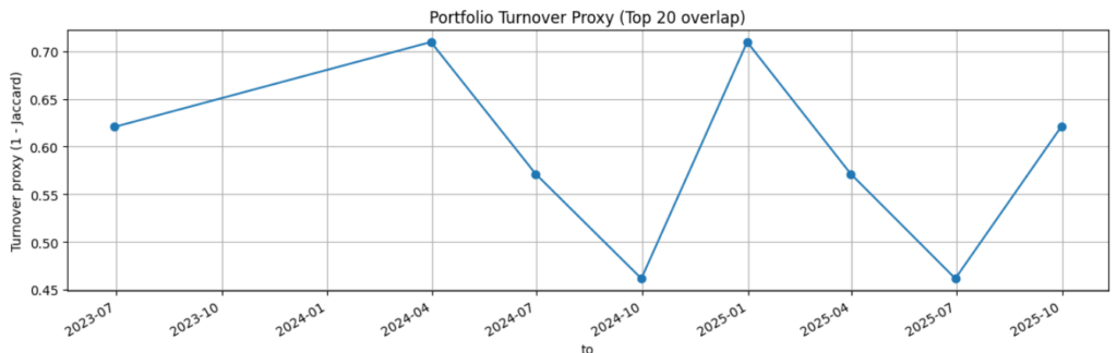
- 「回転率」=どれくらい入れ替えてる?
- 新規追加”と“消滅”を抽出
- 集中度(HHI)と累積比率
- 相関マトリクス
- ポートフォリオのボラティリティ
- VaR(Value at Risk)とポートフォリオリターンの分布
- ポートフォリオ構築によるリスク削減
- リスク寄与度の可視化
- ベンチマークとの比較
- アルファ・ベータ分析
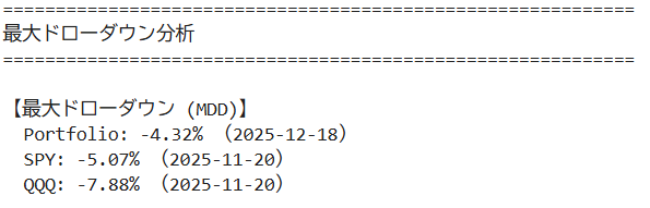
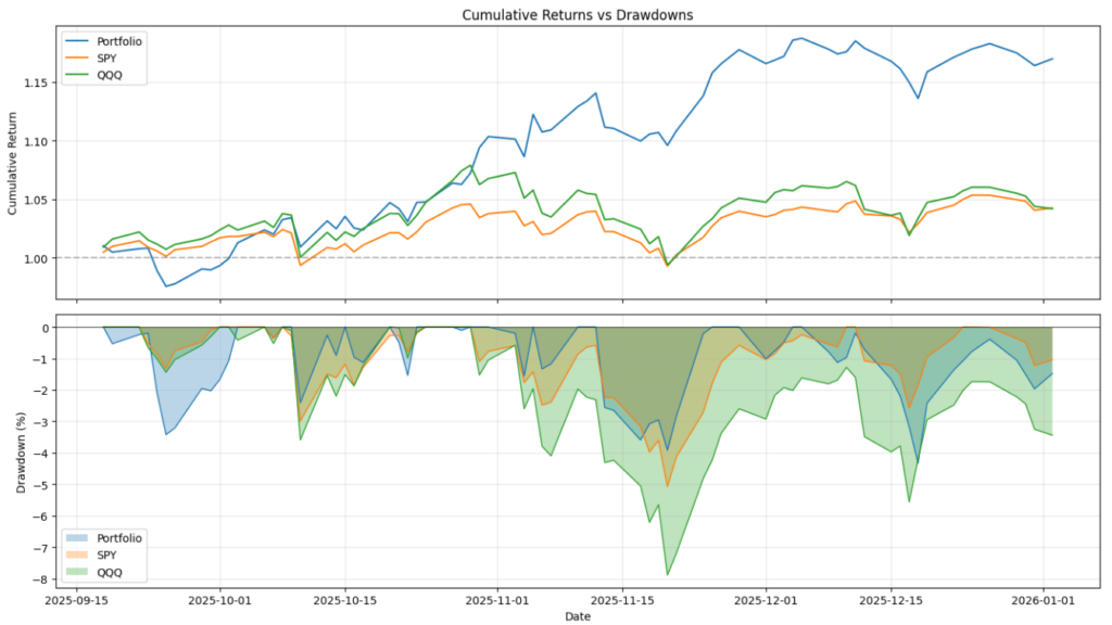
- ドローダウンの計算(直近)
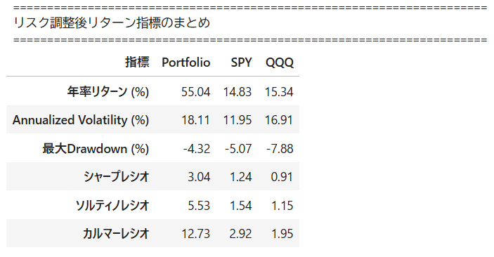
- リスク調整後のリターン指標
- 他の著名投資家との比較
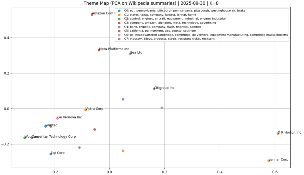
- テーマ抽出
ライブラリのインポートと設定
import time
import json
import re
from datetime import datetime, timezone
from pathlib import Path

import requests
import pandas as pd
import matplotlib.pyplot as plt

pd.set_option("display.max_rows", 200)
pd.set_option("display.max_columns", 200)
パラメータ設定
SEC EDGARからデータを取得するための設定値を定義します。
メルアドの設定を忘れずに。
# ===== Parameters =====
CIK = "0001536411"  # Duquesne Family Office LLC
FORM_TYPE = "13F-HR"

# ↓あなたのメルアドを設定してね。
USER_AGENT = "research-notebook (contact: ここにあなたのメルアドを書く)"

# Throttle requests a bit (SEC guidance references a max request rate; be polite).
SLEEP_SECONDS = 0.2

# Output
OUTDIR = Path("output")
OUTDIR.mkdir(exist_ok=True)
関数の定義
SEC EDGARへのリクエスト送信、CIK/アクセッション番号の整形、最新の13Fファイル検索、情報テーブルファイルの特定などの関数を定義します。
def sec_get(url: str, *, headers: dict | None = None, sleep: float = SLEEP_SECONDS) -> requests.Response:
    h = {"User-Agent": USER_AGENT, "Accept-Encoding": "gzip, deflate"}
    if headers:
        h.update(headers)
    r = requests.get(url, headers=h, timeout=30)
    time.sleep(sleep)
    r.raise_for_status()
    return r

def cik_no_leading_zeros(cik: str) -> str:
    return str(int(cik))

def accession_no_nodashes(accession_no: str) -> str:
    return accession_no.replace("-", "")

def find_latest_form(submissions_json: dict, form_type: str) -> dict:
    """Return a dict with accessionNumber, filingDate, reportDate for the latest matching form."""
    recent = submissions_json.get("filings", {}).get("recent", {})
    forms = recent.get("form", [])
    accs  = recent.get("accessionNumber", [])
    fdates = recent.get("filingDate", [])
    rdates = recent.get("reportDate", [])
    for form, acc, fdate, rdate in zip(forms, accs, fdates, rdates):
        if form == form_type:
            return {"accessionNumber": acc, "filingDate": fdate, "reportDate": rdate}
    raise ValueError(f"No {form_type} found in recent filings for CIK={CIK}")

def get_filing_index_json(cik: str, accession: str) -> dict:
    cik_nz = cik_no_leading_zeros(cik)
    acc_nd = accession_no_nodashes(accession)
    url = f"https://data.sec.gov/submissions/CIK{cik}.json"
    subs = sec_get(url).json()

    index_url = f"https://www.sec.gov/Archives/edgar/data/{cik_nz}/{acc_nd}/index.json"
    idx = sec_get(index_url).json()
    return subs, idx, index_url

def pick_information_table_file(index_json: dict) -> str:
    """Pick the most likely information table XML file from a filing's index.json."""
    files = index_json.get("directory", {}).get("item", [])
    names = [f.get("name", "") for f in files]

    # Prefer XML files that look like the 13F information table.
    candidates = [n for n in names if n.lower().endswith(".xml") and ("infotable" in n.lower() or "informationtable" in n.lower())]
    if candidates:
        return candidates[0]

    # Some filings use .txt for the info table (less common now). Try that as fallback.
    txt_candidates = [n for n in names if n.lower().endswith(".txt") and ("infotable" in n.lower() or "informationtable" in n.lower() or "form13f" in n.lower())]
    if txt_candidates:
        return txt_candidates[0]

    # As a last resort, return the largest XML file (often the info table).
    xmls = [f for f in files if f.get("name", "").lower().endswith(".xml")]
    if not xmls:
        raise ValueError("No XML files found in index.json; cannot locate information table.")
    xmls_sorted = sorted(xmls, key=lambda d: d.get("size", 0), reverse=True)
    return xmls_sorted[0].get("name")
最新の13F-HRファイルを取得
Duquesne Family Officeの最新の13F-HR提出書類を検索します。
# ===== Fetch latest 13F-HR for Duquesne Family Office =====
submissions_url = f"https://data.sec.gov/submissions/CIK{CIK}.json"
submissions = sec_get(submissions_url).json()

latest_filing  = find_latest_form(submissions, FORM_TYPE)
latest_filing
ファイルインデックスと情報テーブルのURL取得
提出書類のインデックスから情報テーブル(保有銘柄リスト)のXMLファイルを特定します。
# ===== Get filing index.json and locate the information table file =====
submissions, filing_index, filing_index_url = get_filing_index_json(CIK, latest_filing["accessionNumber"])
info_file = pick_information_table_file(filing_index)

cik_nz = cik_no_leading_zeros(CIK)
acc_nd = accession_no_nodashes(latest_filing["accessionNumber"])
base_dir = f"https://www.sec.gov/Archives/edgar/data/{cik_nz}/{acc_nd}"

info_url = f"{base_dir}/{info_file}"
(filing_index_url, info_file, info_url)
情報テーブルのXML解析
SEC 13Fの情報テーブルXMLをパースし、DataFrameに変換します。名前空間に対応した複数のXPathを試行します。
# ===== Parse the information table (namespace-safe + no closed-buffer) =====
from io import StringIO

xml_text = sec_get(info_url).text

# Namespace-aware XPath
# default namespace is declared on <informationTable ... xmlns="...">
NS = {"ns": "http://www.sec.gov/edgar/document/thirteenf/informationtable"}

df = None
xpaths = [
    ".//ns:infoTable",                 # 本命: namespace付きinfoTable
    ".//ns:informationTable/ns:infoTable",
    ".//*[local-name()='infoTable']",  # 保険: namespace無視
]

last_err = None
for xp in xpaths:
    try:
        # IMPORTANT: create a fresh StringIO each attempt (avoid "closed file")
        tmp = pd.read_xml(StringIO(xml_text), xpath=xp, namespaces=NS)
        if tmp is not None and len(tmp) > 0:
            df = tmp
            print("Parsed with xpath:", xp)
            break
    except TypeError:
        # pandasの古い版で namespaces 引数が無い場合があるので、その場合はlocal-name()だけでいく
        try:
            tmp = pd.read_xml(StringIO(xml_text), xpath=".//*[local-name()='infoTable']")
            if tmp is not None and len(tmp) > 0:
                df = tmp
                print("Parsed with xpath: local-name() fallback")
                break
        except Exception as e:
            last_err = e
    except Exception as e:
        last_err = e

if df is None or df.empty:
    raise ValueError(f"Could not parse infoTable. Last error: {last_err}")

df.head()
データクリーニングとウェイト計算
カラム名を正規化し、各銘柄のポートフォリオ比率(ウェイト)を算出します。
# Normalize column names (SEC uses names like: nameOfIssuer, titleOfClass, cusip, value, sshPrnamt, sshPrnamtType, putCall, investmentDiscretion, etc.)
df.columns = [c.strip() for c in df.columns]

# 'value' is typically reported in thousands of dollars (x$1000).
# Convert to numeric safely.
if "value" not in df.columns:
    raise ValueError(f"'value' column not found. Columns: {list(df.columns)}")

df["value"] = pd.to_numeric(df["value"], errors="coerce")
df = df.dropna(subset=["value"]).copy()

total_value = df["value"].sum()
df["weight"] = df["value"] / total_value

# A nicer display table
cols = [c for c in ["nameOfIssuer", "titleOfClass", "cusip", "sshPrnamt", "sshPrnamtType", "value", "weight"] if c in df.columns]
out = df[cols].sort_values("weight", ascending=False).reset_index(drop=True)

out.head(20)
過去の13Fデータ取得
時系列分析のため、過去の13F提出書類から保有銘柄の履歴データを取得します。
# ===== 過去の13Fデータを取得 =====
def fetch_all_13f_filings(cik: str, form_type: str = "13F-HR", max_filings: int = 12) -> list:
    """過去の13F提出書類リストを取得"""
    subs_url = f"https://data.sec.gov/submissions/CIK{cik}.json"
    subs = sec_get(subs_url).json()

    recent = subs.get("filings", {}).get("recent", {})
    forms = recent.get("form", [])
    accs = recent.get("accessionNumber", [])
    fdates = recent.get("filingDate", [])
    rdates = recent.get("reportDate", [])

    filings = []
    for form, acc, fdate, rdate in zip(forms, accs, fdates, rdates):
        if form == form_type:
            filings.append({
                "accessionNumber": acc,
                "filingDate": fdate,
                "reportDate": rdate
            })
            if len(filings) >= max_filings:
                break
    return filings

def fetch_13f_holdings(cik: str, accession: str) -> pd.DataFrame:
    """指定の13Fから保有銘柄を取得"""
    try:
        cik_nz = cik_no_leading_zeros(cik)
        acc_nd = accession_no_nodashes(accession)

        index_url = f"https://www.sec.gov/Archives/edgar/data/{cik_nz}/{acc_nd}/index.json"
        idx = sec_get(index_url).json()
        info_file = pick_information_table_file(idx)

        info_url = f"https://www.sec.gov/Archives/edgar/data/{cik_nz}/{acc_nd}/{info_file}"
        xml_text = sec_get(info_url).text

        NS = {"ns": "http://www.sec.gov/edgar/document/thirteenf/informationtable"}
        for xp in [".//ns:infoTable", ".//*[local-name()='infoTable']"]:
            try:
                tmp = pd.read_xml(StringIO(xml_text), xpath=xp, namespaces=NS)
                if tmp is not None and len(tmp) > 0:
                    return tmp
            except:
                continue
    except Exception as e:
        print(f"  Error: {e}")
    return pd.DataFrame()

# 過去の13Fを取得
print("過去の13Fデータを取得中...")
filings = fetch_all_13f_filings(CIK, max_filings=12)
print(f"取得対象: {len(filings)} Quarter分")

hist_list = []
for f in filings:
    print(f"  {f['reportDate']}...", end=" ")
    holdings = fetch_13f_holdings(CIK, f["accessionNumber"])
    if not holdings.empty:
        holdings["reportDate"] = pd.to_datetime(f["reportDate"])
        holdings["filingDate"] = f["filingDate"]
        hist_list.append(holdings)
        print(f"OK ({len(holdings)} holdings)")
    else:
        print("Failed")

if hist_list:
    hist = pd.concat(hist_list, ignore_index=True)
    print(f"\n取得完了: {len(hist)} 件、{hist['reportDate'].nunique()} Quarter分")
else:
    hist = pd.DataFrame()
    print("データ取得に失敗しました")
Top N の比率推移
ポートフォリオに占めるTop N銘柄の割合の推移をプロットします。
# ===== Top holdings weight over time (robust) =====
import numpy as np

hist2 = hist.copy()
hist2["value"] = pd.to_numeric(hist2["value"], errors="coerce")
hist2 = hist2.dropna(subset=["value"]).copy()

grouped = (
    hist2.groupby(["reportDate", "nameOfIssuer"], as_index=False)["value"]
    .sum()
)

# 最新Quarterの上位10銘柄をトラック
recent_date = grouped["reportDate"].max()
topN = 10
top_names = (
    grouped[grouped["reportDate"] == recent_date]
    .sort_values("value", ascending=False)
    .head(topN)["nameOfIssuer"]
    .tolist()
)

plotdf = (
    grouped[grouped["nameOfIssuer"].isin(top_names)]
    .pivot(index="reportDate", columns="nameOfIssuer", values="value")
    .sort_index()
)

# weight化(%)
plotw = plotdf.div(plotdf.sum(axis=1), axis=0) * 100

ax = plotw.plot(figsize=(12,6), marker="o")
ax.set_ylabel("Weight (%)")
ax.set_title(f"Duquesne 13F Top {topN} Holdings Weight Over Time")
ax.grid(True)
plt.tight_layout()
plt.show()

display(plotw.tail(3))
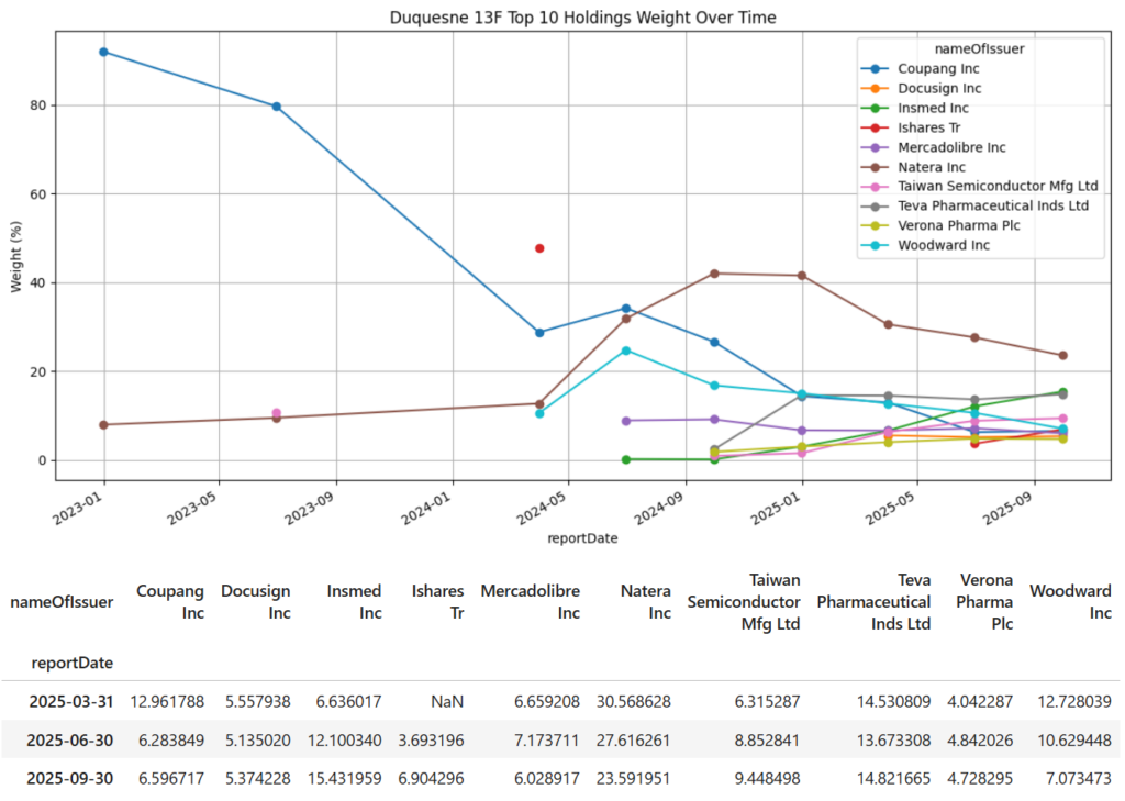
このように表示されます。Coupang Inc(韓国のAmazonと言われる企業。NYSEに上場してる)をガッツリ減らしてるのが一目瞭然。
Quarterごとの売買金額
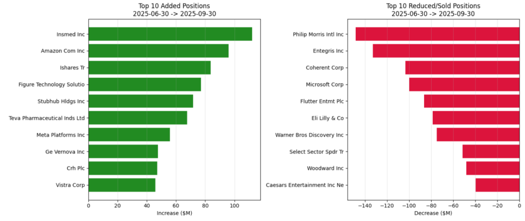
ようやく本丸です。前四半期から増やした銘柄、減らした銘柄をチェックします。
# ===== ポジション変化の計算 =====
# hist2は既にQuarterごとのデータを含んでいる前提

# 各Quarterの銘柄別保有額をピボット
position_pivot = (
    hist2.groupby(["reportDate", "nameOfIssuer"])["value"]
    .sum()
    .unstack(fill_value=0)
)

# Quarter間の差分(変化額)を計算
position_change = position_pivot.diff()

# 最新2Quarterの変化を分析
dates = sorted(position_pivot.index)
if len(dates) >= 2:
    latest_change = position_change.loc[dates[-1]]

    # 買い増し上位
    top_buys = latest_change.nlargest(10)
    # 売却上位
    top_sells = latest_change.nsmallest(10)

    print(f"=" * 60)
    print(f"ポジション変化: {dates[-2].date()} → {dates[-1].date()}")
    print(f"=" * 60)

    print(f"\n【買い増し上位10銘柄】(単位: $1000)")
    display(pd.DataFrame({
        "銘柄": top_buys.index,
        "増加額 ($K)": top_buys.values.astype(int),
        "Increase ($M)": (top_buys.values / 1000).round(1)
    }).reset_index(drop=True))

    print(f"\n【売却/減少上位10銘柄】(単位: $1000)")
    display(pd.DataFrame({
        "銘柄": top_sells.index,
        "減少額 ($K)": top_sells.values.astype(int),
        "Decrease ($M)": (top_sells.values / 1000).round(1)
    }).reset_index(drop=True))
プロットします。
# ===== 売買金額の可視化 =====
fig, axes = plt.subplots(1, 2, figsize=(14, 6))

# 買い増し
ax1 = axes[0]
colors1 = ["forestgreen" if v > 0 else "gray" for v in top_buys.values]
ax1.barh(range(len(top_buys)), top_buys.values / 1000, color=colors1)
ax1.set_yticks(range(len(top_buys)))
ax1.set_yticklabels(top_buys.index)
ax1.set_xlabel("Increase ($M)")
ax1.set_title(f"Top 10 Added Positions\n{dates[-2].date()} -> {dates[-1].date()}")
ax1.grid(True, axis="x", alpha=0.3)
ax1.invert_yaxis()

# 売却
ax2 = axes[1]
colors2 = ["crimson" if v < 0 else "gray" for v in top_sells.values]
ax2.barh(range(len(top_sells)), top_sells.values / 1000, color=colors2)
ax2.set_yticks(range(len(top_sells)))
ax2.set_yticklabels(top_sells.index)
ax2.set_xlabel("Decrease ($M)")
ax2.set_title(f"Top 10 Reduced/Sold Positions\n{dates[-2].date()} -> {dates[-1].date()}")
ax2.grid(True, axis="x", alpha=0.3)
ax2.invert_yaxis()

plt.tight_layout()
plt.show()
以下のように表示されます。
冒頭のnote記事はこのようにForm-13Fから情報を取得、加工して作成しています。
以降、色々と深堀りしてみる。ソースはこちら↓

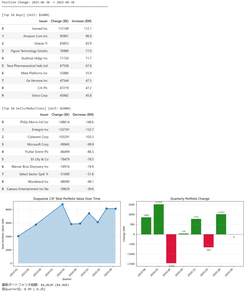
ポートフォリオ総額の推移
上位保有銘柄の可視化(比率と金額)
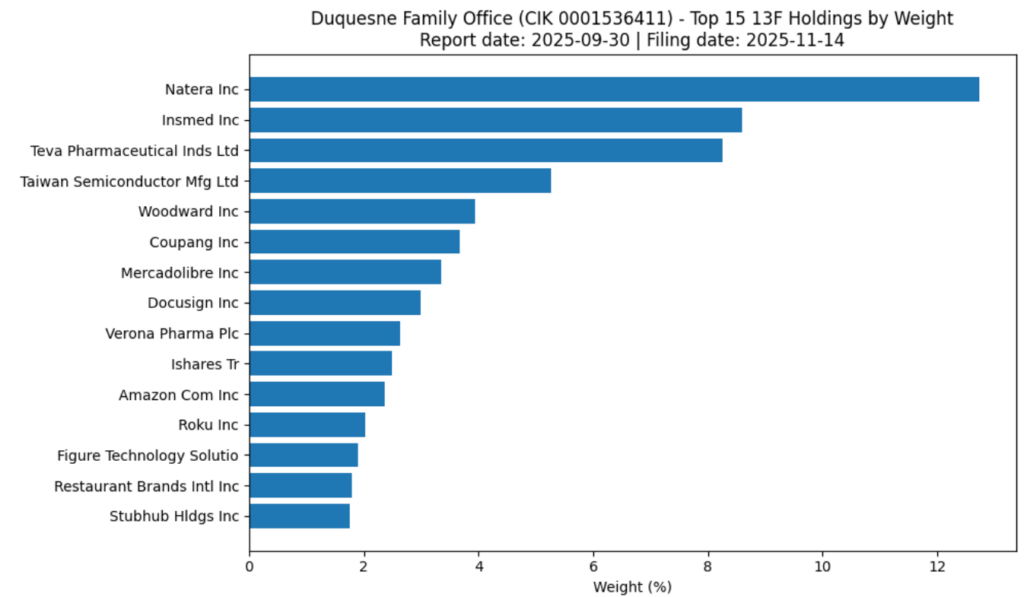
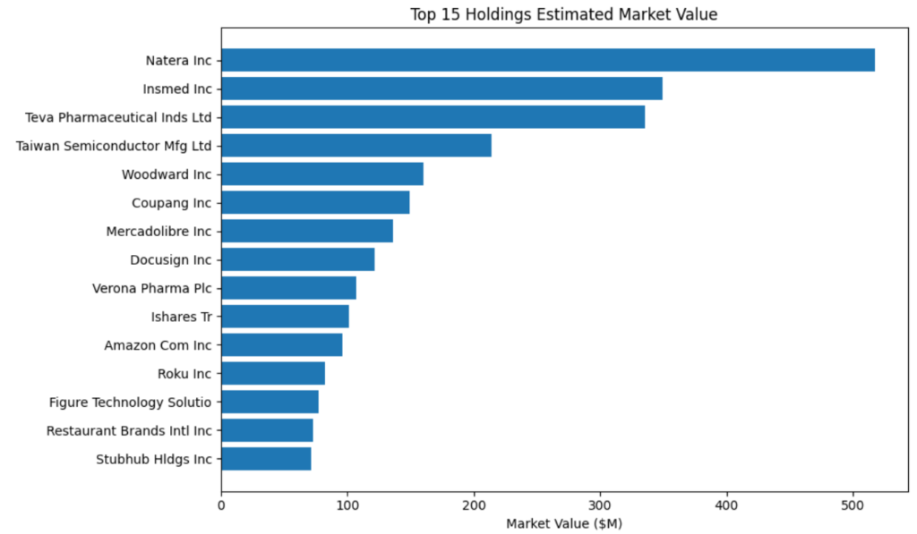
「回転率」=どれくらい入れ替えてる?
新規追加”と“消滅”を抽出

集中度(HHI)と累積比率
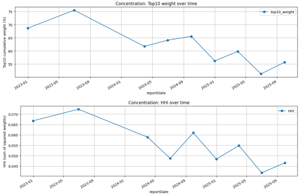
1. 全体トレンド:集中から分散へ
- 2023年6月をピークにTop10比率は75.5% → 51.3%(2025年6月)へ約24ポイント低下
- HHIも0.072 → 0.042と約40%減少
- Druckenmillerは過去2年で明確に分散化を進めている
2. HHIの解釈
- HHI 0.04〜0.07の範囲は「中程度の集中」に該当
- 完全分散(100銘柄均等)ならHHI=0.01、1銘柄集中ならHHI=1.0
- 現在のHHI≈0.045は、実質的に約22銘柄に均等配分した場合と同等(1/0.045≈22)
3. 投資スタイルの変化
- 2023年前半:高確信度の集中投資(「Big Bet」スタイル)
- 2024年以降:リスク分散を重視した慎重なポジショニング
- 市場の不確実性増大に対応し、コンビクションを分散させた可能性
4. 直近の動き(2025年6月→9月)
- Top10比率が51.3%→55.7%へ微増
- 特定銘柄への再集中の兆候があるか、今後のFilingで要注視
5.まとめ
Druckenmillerは従来「少数銘柄に大きく張る」スタイルで知られていたが、2024-2025年にかけてポートフォリオを意図的に分散化。これは:
- マクロ環境の不透明さ
- 金利・インフレの先行き不確実性
- 特定セクター(AI関連など)の過熱感
などに対するリスク管理の表れか。
相関マトリクス
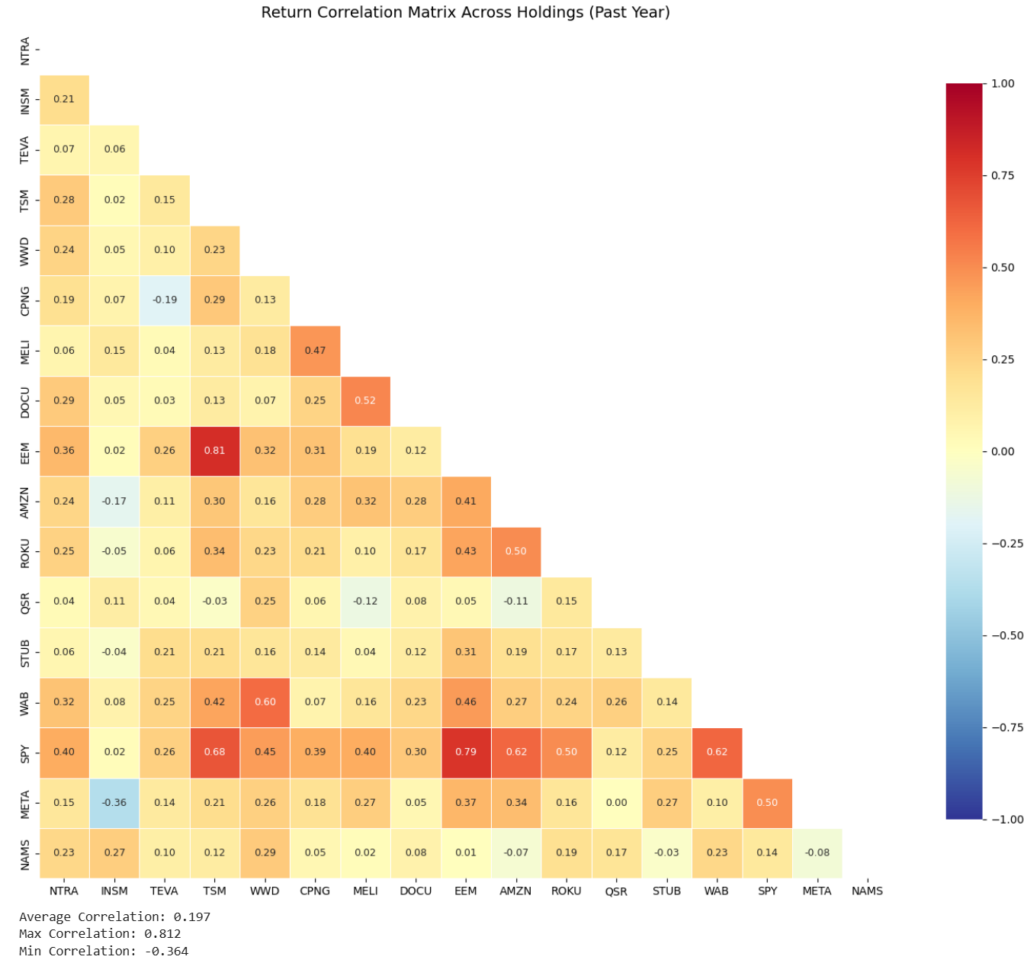
Druckenmillerの「相関を買わない」哲学がよく反映されている。
1. 低い平均相関(0.197)=優れた分散効果
- 平均相関0.2未満は非常に良好な分散を示す
- 銘柄間の値動きが独立しており、同時に下落するリスクが低い
- Druckenmillerが意図的に低相関の銘柄を選択している証拠
2. 最大相関0.812の解釈
- 最も相関が高いペアは恐らく:
- テック大型株同士(META-AMZN、TSM-META等)
- バイオ株同士(NTRA-INSM等)
- 0.8超でも「同一セクター内」ならしゃーなし?
- ポートフォリオ全体への影響は限定的(ウェイト分散により)
3. 負の相関(-0.364)の存在
- ヘッジ効果を持つ銘柄ペアが存在
- 市場下落時に逆行する銘柄がある
- 考えられる負相関ペア:
- TEVA(ディフェンシブ製薬)vs 成長株
- EEM(新興国)vs 米国テック株
ポートフォリオのボラティリティ
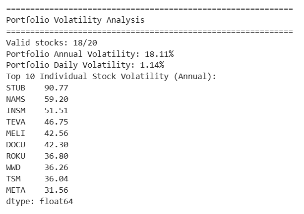
ウェイトも出せばよかったんですが、以下のようになていて、ボラがデカくなりそうなものは低ウェイトにしている。上手ですな。
| 銘柄 | ボラティリティ | ウェイト | 特徴 |
|---|---|---|---|
| STUB | 90.77% | 1.8% | IPO直後、超高ボラ |
| NAMS | 59.20% | 1.3% | 小型バイオ |
| INSM | 51.51% | 8.6% | バイオ(高ウェイト注意) |
| TEVA | 46.75% | 8.3% | 製薬(リストラ中) |
| MELI | 42.56% | 3.4% | 中南米EC |
| DOCU | 42.30% | 3.0% | SaaS成長株 |
| ROKU | 36.80% | 2.0% | ストリーミング |
| WWD | 36.26% | 3.9% | 航空宇宙部品 |
| TSM | 36.04% | 5.3% | 半導体(地政学リスク) |
| META | 31.56% | 1.4% | ビッグテック |
VaR(Value at Risk)とポートフォリオリターンの分布
[Parametric VaR (Normal Distribution)]
95% VaR: -1.66% (1-in-20 day loss)
99% VaR: -2.44% (1-in-100 day loss)
[Historical VaR]
95% VaR: -1.35%
99% VaR: -2.45%
[For $100M Portfolio]
95% Daily VaR: $1,658,391
99% Daily VaR: $2,435,980
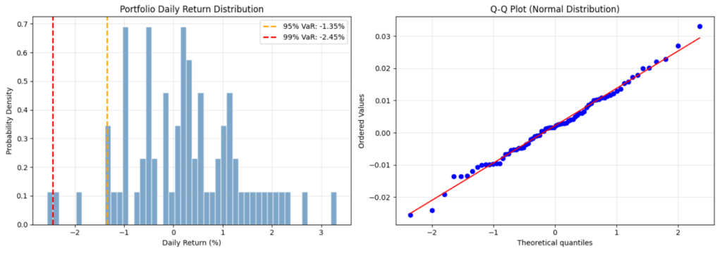
数値の比較:
Parametric (正規分布仮定): -2.44%
Historical (実績ベース): -2.45%
直近の保有銘柄の価格変動は「素直な分布」をしている(テールリスクが顕在化していない)。
この一致は、「計算対象期間において、保有銘柄が極端な暴落(ブラックスワン的イベント)を起こしておらず、比較的高いボラティリティの中で安定して推移していた」ことを示唆します。あるいは、保有銘柄(例えばNVIDIAやMicrosoftなどの大型テック)の流動性が高く、市場全体の動きに連動しやすい構成になっている可能性があります。
補足:
通常、ヘッジファンドのポートフォリオは「ファットテール(正規分布よりも極端な損益が出やすい)」傾向にあり、Historical VaRの方が悪く出ることが多いです。
QQプロット(グラフ右側)でもリターンが正規分布に従っており、ファットテール(極端な損失)が少ないことが分かる(もちろん極端な利益も少ない)。
ポートフォリオ構築によるリスク削減
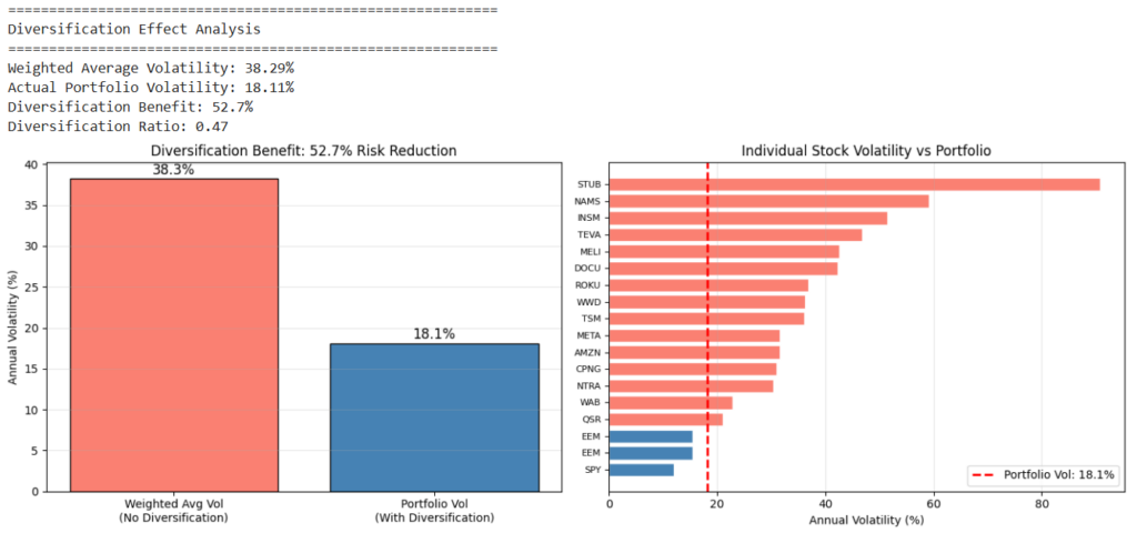
ボラが38.29%から18.11%に削減できてる。リターンを確保した上でのリスク削減比率 0.47はかなり優秀。
リスク寄与度の可視化
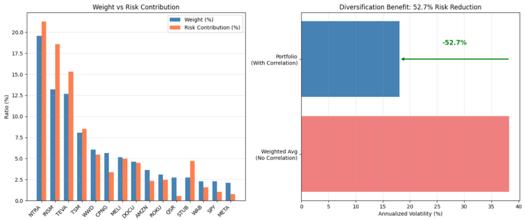
理想的なリスクパリティ(全銘柄のリスク寄与が均等)とは乖離があり、純な「高ボラ=小さく」ではなく、確信度×ボラティリティでサイズ決定と思われる。この辺がDruckenmillerが年30%の利回りを長期に渡って出せる所以やろな。
ベンチマークとの比較
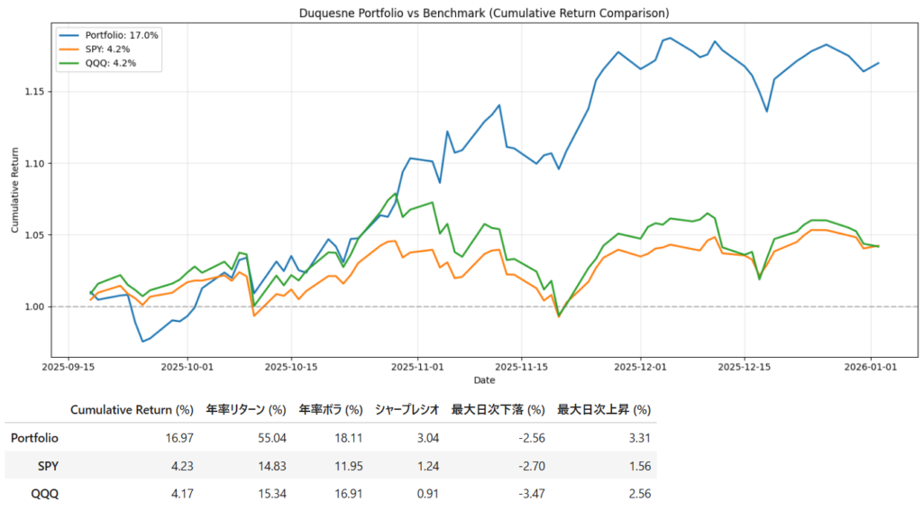
優秀。
アルファ・ベータ分析
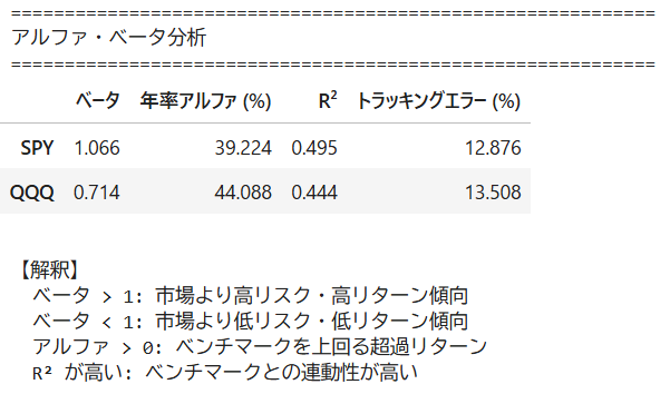
- 「市場と同程度のリスクで、市場を大幅に上回るリターン」 を実現
- 低R²と高トラッキングエラーは真のアクティブ運用の証拠
- QQQより低ベータなのは、テック一辺倒を避けた分散の結果かな?
- アルファの源泉は銘柄選択力(バイオ/新興国の選定眼)
回帰プロット
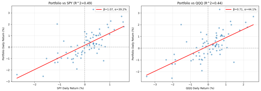
優秀。
- 回帰線が原点より上を通過(切片が大きく正)
- 散布図の点が回帰線の上側に偏在する傾向
- 市場下落時でも踏みとどまる点(左上象限)の存在(多くはないが)
ドローダウンの計算(直近)
リスク調整後のリターン指標
他の著名投資家との比較

テーマ抽出
どのテーマ(カテゴリ)の銘柄を保有しているか?
以上です。


コメント